How to do convolutions with doubly blocked Toeplitz matrices

A few weeks ago, Jamie (@neworderofjamie) asked me on the chat whether I knew what doubly blocked Toeplitz matrices are and how they implement convolutions. I had no clue. Since then we have implemented convolutions using doubly blocked Toeplitz matrices in GeNN and found them to be extremely useful and efficient. 1 In this software blog I will give a brief overview on the why and how convolutions relate to doubly blocked Toeplitz matrices. My blog is based on Ali Salehi's tutorial Convolution as Matrix Multiplication but updated to use machine-learning rather than signal-processing conventions and I am trying to avoid using too many unusual ways of re-arranging rows and columns.

The why

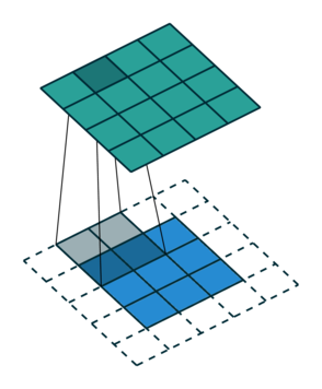
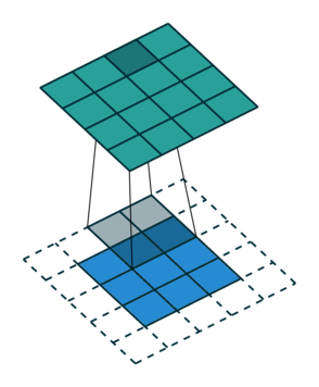
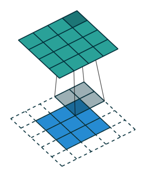
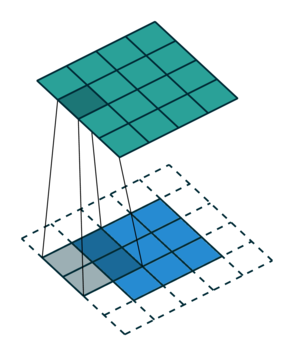
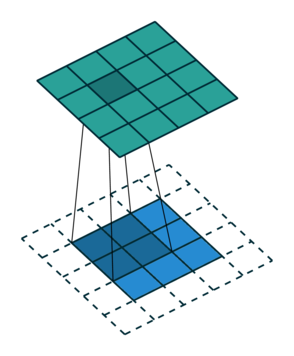
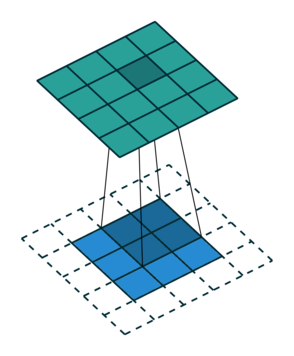
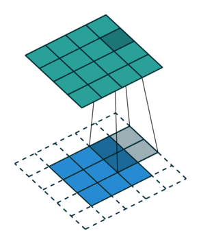
Let us consider the convolution of a \(2\times 2\) kernel with a \(3\times 3\) layer. We denote the kernel as \[ K= \left(\matrix{ k_{11} & k_{12} \cr k_{21} & k_{22}}\right) \] and the layer as \[ I= \left(\matrix{ i_{11} & i_{12} & i_{13} \cr i_{21} & i_{22} & i_{23} \cr i_{31} & i_{32} & i_{33} } \right). \] Then the convolution in the machine learning use of the term is calculating the cross-correlation of the kernel "moving across" the layer as illustrated below. The layer \(I\) is in blue, the kernel \(K\) in grey and the result \(R\) in green.

1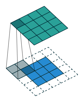
\(r_{11}\)	\(r_{12}\)	\(r_{13}\)	\(3_{14}\)

For the first non-zero entry at \((1,1)\) of the result matrix \(R\), we therefore have \(r_{11} = k_{22} i_{11}\). Then the kernel moves one over and \(r_{12} = k_{21}i_{11} + k_{22} i_{12}\). Then, \(r_{13} = k_{21}i_{12} + k_{22} i_{13}\) and \(r_{14} = k_{21}i_{13} \).

\(r_{21}\)	\(r_{22}\)	\(r_{23}\)	\(r_{24}\)

So, for the second row, \(r_{21} = k_{12} i_{11} + k_{22} i_{21} \), move one over, \(r_{22} = k_{11} i_{11} + k_{12} i_{12} + k_{21} i_{21} + k_{22} i_{22} \), one more to the right, \(r_{23} = k_{11}i_{12} + k_{12} i_{13} + k_{21} i_{22} + k_{22} i_{23} \), and finally \(r_{24} = k_{11}i_{13} + k_{21} i_{23} \).

It works similar for the remaining two rows.

If we unroll the layer \(I\) row-wise into a column vector \(I_\text{col}\), \[ I_\text{col} = \left( \matrix{ i_{11} \cr i_{12} \cr i_{13} \cr i_{21} \cr i_{22} \cr i_{23} \cr i_{31} \cr i_{32} \cr i_{33} } \right), \] then we can express this as a matrix-vector multiplication of a matrix formed from the entries of the kernel \(K\) and the vector\(I_\text{col}\), \[ \left(\matrix{ k_{22} & 0 & 0 & 0 & 0 & 0 & 0 & 0 & 0 \cr k_{21} & k_{22} & 0 & 0 & 0 & 0 & 0 & 0 & 0 \cr 0 & k_{21} & k_{22} & 0 & 0 & 0 & 0 & 0 & 0 \cr 0 & 0 & k_{21} & k_{22} & 0 & 0 & 0 & 0 & 0 \cr k_{12} & 0 & 0 & k_{22} & 0 & 0 & 0 & 0 & 0 \cr k_{11} & k_{12} & 0 & k_{21} & k_{22} & 0 & 0 & 0 & 0 \cr 0 & k_{11} & k_{12} & 0 & k_{21} & k_{22} & 0 & 0 & 0 \cr 0 & 0 & k_{11} & 0 & 0 & k_{21} & 0 & 0 & 0 \cr 0 & 0 & 0 & k_{12} & 0 & 0 & k_{22} & 0 & 0 \cr 0 & 0 & 0 & k_{11} & k_{12} & 0 & k_{21} & k_{22} & 0 \cr 0 & 0 & 0 & 0 & k_{11} & k_{12} & 0 & k_{21} & k_{22} \cr 0 & 0 & 0 & 0 & 0 & k_{11} & 0 & 0 & k_{21} \cr 0 & 0 & 0 & 0 & 0 & 0 & k_{12} & 0 & 0 \cr 0 & 0 & 0 & 0 & 0 & 0 & k_{11} & k_{12} & 0 \cr 0 & 0 & 0 & 0 & 0 & 0 & 0 & k_{11} & k_{12} \cr 0 & 0 & 0 & 0 & 0 & 0 & 0 & 0 & k_{11} }\right) \cdot \left(\matrix{ i_{11} \cr i_{12} \cr i_{13} \cr i_{21} \cr i_{22} \cr i_{23} \cr i_{31} \cr i_{32} \cr i_{33}} \right) \]

Now one can already see that the matrix formed from the kernel entries has a very peculiar shape - the shape of a doubly blocked Toeplitz matrix

Doubly blocked Toeplitz matrix

A Toeplitz matrix is a matrix where the values along all diagonals are constant, i.e.

\[ \left( \matrix{ a_{0} & a_{-1} & a_{-2} & \cdots & \cdots & \cdots & a_{-(N-1)} \cr a_{1} & a_{0} & a_{-1} & a_{-2} & & & \vdots \cr a_{2} & a_{1} & a_{0} & a_{-1} & & & \vdots \cr \vdots & \ddots & \ddots & \ddots & \ddots & \ddots & & \vdots \cr \vdots & & & \ddots & a_{0} & a_{-1} & a_{-2} \cr \vdots & & & & a_{1} & a_{0} & a_{-1} \cr a_{M-1} & \cdots & \cdots & \cdots & a_{2} & a_{1} & a_{0} } \right) . \]

Furthermore, if we build a matrix \(A\) out of Toeplitz sub-matrices \(A_{k}\) and the structure of \(A\) with respect to these submatrices is also Toeplitz:

\[ A = \left( \matrix{ A_{0} & A_{-1} & \cdots & A_{-(L-1)} \cr A_{1} & A_{0} & \cdots & A_{-(L-2)} \cr \vdots & \vdots & \ddots & \vdots \cr A_{K} & A_{K-1} & \cdots & A_{0}} \right), \]

then, this matrix is called a doubly-blocked Toeplitz matrix. A standard way to generate a Toeplitz matrix from a vector \(v\) is to use \(v\) as the first column vector, then make one cyclic permutation and use it as the second column vector and so on.

The method

As we have seen on the example above, 2D convolution operations can be expressed as multiplication by a doubly-blocked Toeplitz matrix. As a general method, applied to the example above, to convolve \(K\) with \(I\), we first flip \(K\) across the horizontal and vertical axis and pad it to the output size \((I_\text{height} + K_\text{height} - 1) \times (I_\text{width} + K_\text{width} - 1)\) of the convolution. For instance, here, the \(3 \times 3\) layer \(I\) covolved by \(K\) above, leads to output size \(4 \times 4\). Depending on the padding mode used by the convolution, typically, only part of this output is actually required. The flipped and padded kernel \(K\) from above is \[ K_\text{pad}= \left( \matrix{ k_{22} & k_{21} & 0 & 0 \cr k_{12} & k_{11} & 0 & 0 \cr 0 & 0 & 0 & 0 \cr 0 & 0 & 0 & 0 } \right) \]

We then convert each row vector of this matrix into Toeplitz matrices \(F_i\) as described above: \[ F_0= \left( \matrix{ k_{22} & 0 & 0 \cr k_{21} & k_{22} & 0 \cr 0 & k_{21} & k_{22} \cr 0 & 0 & k_{21}} \right) \quad F_1= \left( \matrix{ k_{12} & 0 & 0 \cr k_{11} & k_{12} & 0 \cr 0 & k_{11} & k_{12} \cr 0 & 0 & k_{11}} \right) \] \[ F_2= \left( \matrix{ 0 & 0 & 0 \cr 0 & 0 & 0 \cr 0 & 0 & 0 \cr 0 & 0 & 0} \right) \quad F_3= \left( \matrix{ 0 & 0 & 0 \cr 0 & 0 & 0 \cr 0 & 0 & 0 \cr 0 & 0 & 0} \right) \] and, finally, assemble these into a doubly blocked Toeplitz matrix \(F\):

\[ F= \left( \matrix{ F_0 & F_3 & F_2 \cr F_1 & F_0 & F_3 \cr F_2 & F_1 & F_0 \cr F_3 & F_2 & F_1 } \right) \]

The convolution of \(K\) with \(I\) is then given by multiplying F from the left onto \(I_\text{col}\) as defined above, \[ R_{\text{col}} = F \cdot I \quad \Leftrightarrow \quad R_{\text{col},j}= \sum_i F_{ji}I_i \]

Finally, \(R_{\text{col}}\) can be reinterpreted as the output matrix \(R\) by arranging its entries row-wise in a \(4\times 4\) matrix.

There we have it - convolution (in the machine learning sense, i.e. corss-correlation) of a kernel \(K\) with a layer \(I\) expressed as the product of a doubly blocked Toeplitz matrix derived from \(K\) with the column vector of the row-wise unrolled entries from \(I\).

The following python function is a simple implementation of this method

import numpy as np
from scipy.linalg import toeplitz

def convolution(I, K, verbose= False):
    # flip the kernel
    K= np.fliplr(np.flipud(K))
    # calculate sizes
    K_row_num, K_col_num= K.shape
    I_row_num, I_col_num= I.shape
    R_row_num= K_row_num+I_row_num-1
    R_col_num= K_col_num+I_col_num-1
    # pad the kernel
    K_pad= np.pad(K, ((0,R_row_num - K_row_num),
                      (0,R_col_num - K_col_num)), 
                  'constant', constant_values= 0)
    if verbose:
        print("padded kernel= \n", K_pad)
    # Assemble the list of Toeplitz matrices F_i
    toeplitz_list= []
    for i in range(R_row_num):
        c= K_pad[i,:]
        r= np.r_[c[0],np.zeros(I_col_num-1)]
        toeplitz_list.append(toeplitz(c,r).copy())
    if verbose:
        print("Toeplitz list= \n", toeplitz_list)
    # make a matrix with the indices of the block F_i 
    # of the doubly blocked Toeplitz matrix
    c = np.array(range(R_row_num))
    r = np.r_[c[0], c[-1:1:-1]]
    doubly_indices = np.array(toeplitz(c,r).copy())
    if verbose:
        print("doubly_indices= \n", doubly_indices)
    # assemble the doubly blocked toeplitz matrix
    toeplitz_m= []
    for i in range(R_row_num):
        row= []
        for j in range(I_row_num):
            row.append(toeplitz_list[doubly_indices[i,j]])
        row=np.hstack(row)
        toeplitz_m.append(row)
    toeplitz_m= np.vstack(toeplitz_m)
    if verbose:
        print("Toeplitz matrix= \n",toeplitz_m)
    # make layer into column vector
    I_col= I.flatten()
    if verbose:
        print("I_col= ", I_col)
    R = np.matmul(toeplitz_m, I_col)
    if verbose:
        print('R as vector= \n', R)
    R= R.reshape(R_row_num, R_col_num)
    if verbose: 
        print('R as matrix= \n', R)
    return R

To test, one can, for instance, use

# kernel
K= np.array([[10,20],[30,40]])
# layer
I= np.array([[1,2,3],[4,5,6]])
R= convolution(I, K, verbose= True)

The output would then be

padded kernel= 
 [[40 30  0  0]
 [20 10  0  0]
 [ 0  0  0  0]]
Toeplitz list= 
 [array([[40.,  0.,  0.],
       [30., 40.,  0.],
       [ 0., 30., 40.],
       [ 0.,  0., 30.]]), array([[20.,  0.,  0.],
       [10., 20.,  0.],
       [ 0., 10., 20.],
       [ 0.,  0., 10.]]), array([[0., 0., 0.],
       [0., 0., 0.],
       [0., 0., 0.],
       [0., 0., 0.]])]
doubly_indices= 
 [[0 2]
 [1 0]
 [2 1]]
Toeplitz matrix= 
 [[40.  0.  0.  0.  0.  0.]
 [30. 40.  0.  0.  0.  0.]
 [ 0. 30. 40.  0.  0.  0.]
 [ 0.  0. 30.  0.  0.  0.]
 [20.  0.  0. 40.  0.  0.]
 [10. 20.  0. 30. 40.  0.]
 [ 0. 10. 20.  0. 30. 40.]
 [ 0.  0. 10.  0.  0. 30.]
 [ 0.  0.  0. 20.  0.  0.]
 [ 0.  0.  0. 10. 20.  0.]
 [ 0.  0.  0.  0. 10. 20.]
 [ 0.  0.  0.  0.  0. 10.]]
I_col=  [1 2 3 4 5 6]
R as vector= 
 [ 40. 110. 180.  90. 180. 370. 470. 210.  80. 140. 170.  60.]
R as matrix= 
 [[ 40. 110. 180.  90.]
 [180. 370. 470. 210.]
 [ 80. 140. 170.  60.]]

Note, that this example is inspired by Salehi's tutorial but because we are calculating the machine learning covolution (cross-correlation) and Salehi the mathematical convolution as used in signal processing, the results are not the same. To generate identical results one can use the doubly flipped kernel,

# kernel
K= np.array([[40,30],[20,10]])
# layer
I= np.array([[1,2,3],[4,5,6]])
R= convolution(I, K, verbose= False)
print("R= \n", R)

and obtain

 R= 
 [[ 10.  40.  70.  60.]
 [ 70. 230. 330. 240.]
 [120. 310. 380. 240.]]

which exactly is Salehi's result.