In this tutorial we will go through step by step instructions how to create and run your first PyGeNN simulation from scratch.

In this tutorial we will use a pre-defined Hodgkin-Huxley neuron model (NeuronModels::TraubMiles) and create a simulation consisting of ten such neurons without any synaptic connections. We will run this simulation on a GPU and plot the results using Matplotlib.

The first step is to create a new Python script. Create a new directory and, within that, create a new empty file called tenHH.py using your favourite text editor, e.g.

>> emacs tenHH.py &

Note: The ">>" in the example code snippets refers to a shell prompt in a unix shell, do not enter them as part of your shell commands.

This Python script will contain the definition of the network model as well as the code to simulate the model and plot the results. First, we need to import some classes from PyGeNN so we can reference them succinctly. Type in your tenHH.py file:

from pygenn.genn_model import GeNNModel

Two standard elements to the model definition are setting the simulation step size, the name of the model and the precision to simulate with:

model = GeNNModel("float", "tenHH")

model.dT = 0.1

Note: With this we have fixed the integration time step to 0.1 in the usual time units. The typical units in GeNN are ms, mV, nF, and μS. Therefore, this defines DT= 0.1 ms.

Making the actual model definition makes use of the pygenn.GeNNModel.add_neuron_population and pygenn.GeNNModel.add_synapse_population member functions of the pygenn.GeNNModel object. The arguments to a call to pygenn.GeNNModel.add_neuron_population are:

pop_name: Unique name of the neuron population
num_neurons: number of neurons in the population
neuron: The type of neuron model. This should either be a string containing the name of a built in model or user-defined neuron type returned by pygenn.genn_model.create_custom_neuron_class (see Neuron models).
param_space: Dictionary containing parameters of this neuron type
var_space: Dictionary containing initial values or initialisation snippets for variables of this neuron type

We first create the parameter and initial variable arrays,

p = {"gNa": 7.15,   # Na conductance in [muS]
     "ENa": 50.0,   # Na equi potential [mV]
     "gK": 1.43,    # K conductance in [muS]
     "EK": -95.0,   # K equi potential [mV] 
     "gl": 0.02672, # leak conductance [muS]
     "El": -63.563, # El: leak equi potential in mV, 
     "C": 0.143}    # membr. capacity density in nF
ini = {"V": -60.0,      # membrane potential
       "m": 0.0529324,  # prob. for Na channel activation
       "h": 0.3176767,  # prob. for not Na channel blocking
       "n": 0.5961207}  # prob. for K channel activation

Note: The comments are obviously only for clarity, they can in principle be omitted.

Having defined the parameter values and initial values we can now create the neuron population,

pop1 = model.add_neuron_population("Pop1", 10, "TraubMiles", p, ini)

This model definition will generate code for simulating ten Hodgkin-Huxley neurons on the a GPU or CPU. The next stage is to write the code that sets up the simulation, does the data handling for input and output and generally defines the numerical experiment to be run. To build your model description into simulation code, simply call pygenn.GeNNModel.build

model.build()

If you have an NVIDIA GPU and CUDA_PATH is correctly configured, this will generate and build CUDA code to simulate your model. If not, it will generate and build C++ code. This completes the model definition in this example. The complete tenHH.py file now should look like this:

from pygenn.genn_model import GeNNModel
model = GeNNModel("float", "tenHH")
model.dT = 0.1
p = {"gNa": 7.15,   # Na conductance in [muS]
     "ENa": 50.0,   # Na equi potential [mV]
     "gK": 1.43,    # K conductance in [muS]
     "EK": -95.0,   # K equi potential [mV] 
     "gl": 0.02672, # leak conductance [muS]
     "El": -63.563, # El: leak equi potential in mV, 
     "C": 0.143}    # membr. capacity density in nF
ini = {"V": -60.0,      # membrane potential
       "m": 0.0529324,  # prob. for Na channel activation
       "h": 0.3176767,  # prob. for not Na channel blocking
       "n": 0.5961207}  # prob. for K channel activation
pop1 = model.add_neuron_population("Pop1", 10, "TraubMiles", p, ini)
model.build()

User Code

The generated code to simulate the model will now have been generated. To make use of this code, we need to load it into PyGeNN:

model.load()

For the purposes of this tutorial we will initially simply run the model for 200ms and print the final neuron variables. To do so, we add:

Note: The pygenn.GeNNModel.t property keeps track of the current simulation time in milliseconds.

while model.t < 200.0

model.step_time()

and we need to copy the result back to the host (this will do nothing if you are running the model on a CPU) before printing it out,

pop1.pull_state_from_device()
v_view = pop1.vars["V"].view
m_view = pop1.vars["m"].view
h_view = pop1.vars["h"].view
n_view = pop1.vars["n"].view
for j in range(10):
    print("%f %f %f %f" % (v_view[j], m_view[j], h_view[j], n_view[j]))

pygenn.NeuronGroup.pull_state_from_device copies all relevant state variables of the neuron group from the GPU to the CPU main memory. We can then get direct access to the host-allocated memory using a 'view' and finally output the results to stdout by looping through all 10 neurons and outputting the state variables via their views.

This completes the first version of the script. The complete tenHH.py file should now look like

from pygenn.genn_model import GeNNModel
model = GeNNModel("float", "tenHH")
model.dT = 0.1
p = {"gNa": 7.15,   # Na conductance in [muS]
     "ENa": 50.0,   # Na equi potential [mV]
     "gK": 1.43,    # K conductance in [muS]
     "EK": -95.0,   # K equi potential [mV] 
     "gl": 0.02672, # leak conductance [muS]
     "El": -63.563, # El: leak equi potential in mV, 
     "C": 0.143}    # membr. capacity density in nF
ini = {"V": -60.0,      # membrane potential
       "m": 0.0529324,  # prob. for Na channel activation
       "h": 0.3176767,  # prob. for not Na channel blocking
       "n": 0.5961207}  # prob. for K channel activation
pop1 = model.add_neuron_population("Pop1", 10, "TraubMiles", p, ini)
model.build()
model.load()
while model.t < 200.0:
    model.step_time()
pop1.pull_state_from_device()
v_view = pop1.vars["V"].view
m_view = pop1.vars["m"].view
h_view = pop1.vars["h"].view
n_view = pop1.vars["n"].view
for j in range(10):
    print("%f %f %f %f" % (v_view[j], m_view[j], h_view[j], n_view[j]))

Running the Simulation

You can now execute your newly-built simulator with

>> python tenHH.py

The output you obtain should look like

-63.305061 0.020786 0.993780 0.049409
-63.305061 0.020786 0.993780 0.049409
-63.305061 0.020786 0.993780 0.049409
-63.305061 0.020786 0.993780 0.049409
-63.305061 0.020786 0.993780 0.049409
-63.305061 0.020786 0.993780 0.049409
-63.305061 0.020786 0.993780 0.049409
-63.305061 0.020786 0.993780 0.049409
-63.305061 0.020786 0.993780 0.049409
-63.305061 0.020786 0.993780 0.049409

Reading

This is not particularly interesting as we are just observing the final value of the membrane potentials. To see what is going on in the meantime, we need to copy intermediate values from the device into a data structure and plot them. This can be done in many ways but one sensible way of doing this is to replace the calls to pygenn.GeNNModel.step_time in tenHH.py with something like this:

v = np.empty((2000, 10))
v_view = pop1.vars["V"].view
while model.t < 200.0:
    model.step_time()
    pop1.pull_var_from_device("V")
    
    v[model.timestep - 1,:]=v_view[:]

You will also need to add:

import numpy as np

to the top of tenHH.py.

Note: The pygenn.GeNNModel.timestep property keeps track of the current simulation timestep count. This is updated at the end of pygenn.GeNNModel.step_time so here, we subtract 1 from it to obtain indices into our array from 0 to 9999.; We switched from using pygenn.NeuronGroup.pull_state_from_device to pygenn.genn_group.NeuronGroup.pull_var_from_device as we are now only interested in the membrane voltage of the neuron.

Finally, if we add:

fig, axis = plt.subplots()
axis.plot(v)
plt.show()

to the bottom of tenHH.py and:

import matplotlib.pyplot as plt

to the top, if you run the simulation again as described above you should observe dynamics like this:

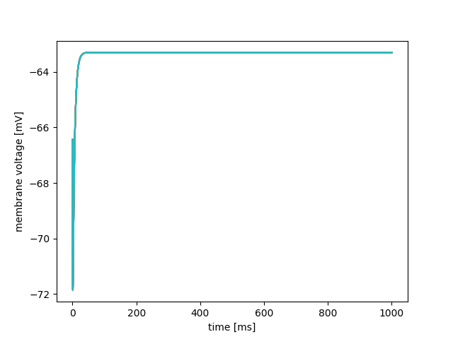
However so far, the neurons are not connected and do not receive input. As the NeuronModels::TraubMiles model is silent in such conditions, the membrane voltages of the 10 neurons will simply drift from the -60mV they were initialised at to their resting potential.

Previous | Top | Next