Adding Kenyon Cells

In this second tutorial we add a large population of Kenyon Cells to the mushroom body and visualize their spiking activity in response to latency coded MNIST digits.

Install PyGeNN wheel from Google Drive

Download wheel file

if "google.colab" in str(get_ipython()):
    #import IPython
    #IPython.core.magics.execution.ExecutionMagics.run.func_defaults[2] = lambda a: a
    #%run "../install_collab.ipynb"
    !pip install gdown --upgrade
    !gdown 1V_GzXUDzcFz9QDIpxAD8QNEglcSipssW
    !pip install pygenn-5.0.0-cp310-cp310-linux_x86_64.whl
    %env CUDA_PATH=/usr/local/cuda

Requirement already satisfied: gdown in /usr/local/lib/python3.10/dist-packages (5.1.0)
Requirement already satisfied: beautifulsoup4 in /usr/local/lib/python3.10/dist-packages (from gdown) (4.12.3)
Requirement already satisfied: filelock in /usr/local/lib/python3.10/dist-packages (from gdown) (3.13.1)
Requirement already satisfied: requests[socks] in /usr/local/lib/python3.10/dist-packages (from gdown) (2.31.0)
Requirement already satisfied: tqdm in /usr/local/lib/python3.10/dist-packages (from gdown) (4.66.2)
Requirement already satisfied: soupsieve>1.2 in /usr/local/lib/python3.10/dist-packages (from beautifulsoup4->gdown) (2.5)
Requirement already satisfied: charset-normalizer<4,>=2 in /usr/local/lib/python3.10/dist-packages (from requests[socks]->gdown) (3.3.2)
Requirement already satisfied: idna<4,>=2.5 in /usr/local/lib/python3.10/dist-packages (from requests[socks]->gdown) (3.6)
Requirement already satisfied: urllib3<3,>=1.21.1 in /usr/local/lib/python3.10/dist-packages (from requests[socks]->gdown) (2.0.7)
Requirement already satisfied: certifi>=2017.4.17 in /usr/local/lib/python3.10/dist-packages (from requests[socks]->gdown) (2024.2.2)
Requirement already satisfied: PySocks!=1.5.7,>=1.5.6 in /usr/local/lib/python3.10/dist-packages (from requests[socks]->gdown) (1.7.1)
Downloading...
From: https://drive.google.com/uc?id=1V_GzXUDzcFz9QDIpxAD8QNEglcSipssW
To: /content/pygenn-5.0.0-cp310-cp310-linux_x86_64.whl
100% 8.29M/8.29M [00:00<00:00, 69.0MB/s]
Processing ./pygenn-5.0.0-cp310-cp310-linux_x86_64.whl
Requirement already satisfied: numpy>=1.17 in /usr/local/lib/python3.10/dist-packages (from pygenn==5.0.0) (1.25.2)
Requirement already satisfied: deprecated in /usr/local/lib/python3.10/dist-packages (from pygenn==5.0.0) (1.2.14)
Requirement already satisfied: psutil in /usr/local/lib/python3.10/dist-packages (from pygenn==5.0.0) (5.9.5)
Requirement already satisfied: wrapt<2,>=1.10 in /usr/local/lib/python3.10/dist-packages (from deprecated->pygenn==5.0.0) (1.14.1)
pygenn is already installed with the same version as the provided wheel. Use --force-reinstall to force an installation of the wheel.
env: CUDA_PATH=/usr/local/cuda

Install MNIST package

!pip install mnist

Collecting mnist
  Downloading mnist-0.2.2-py2.py3-none-any.whl (3.5 kB)
Requirement already satisfied: numpy in /usr/local/lib/python3.10/dist-packages (from mnist) (1.25.2)
Installing collected packages: mnist
Successfully installed mnist-0.2.2

Build tutorial model

Import modules

import mnist
import numpy as np
from copy import copy
from matplotlib import pyplot as plt
from pygenn import (create_current_source_model, init_postsynaptic,
                    init_sparse_connectivity, init_weight_update, GeNNModel)

training_images = mnist.train_images()
training_images = np.reshape(training_images, (training_images.shape[0], -1)).astype(np.float32)

# Reshape and normalise training data
training_images /= np.sum(training_images, axis=1)[:, np.newaxis]

Parameters

Define some model parameters

# Simulation time step
DT = 0.1

# Scaling factor for converting normalised image pixels to input currents (nA)
INPUT_SCALE = 80.0

# Number of Projection Neurons in model (should match image size)
NUM_PN = 784

# Number of Kenyon Cells in model (defines memory capacity)
NUM_KC = 20000

# How long to present each image to model
PRESENT_TIME_MS = 20.0

# Standard LIF neurons parameters
LIF_PARAMS = {
    "C": 0.2,
    "TauM": 20.0,
    "Vrest": -60.0,
    "Vreset": -60.0,
    "Vthresh": -50.0,
    "Ioffset": 0.0,
    "TauRefrac": 2.0}

# We only want PNs to spike once
PN_PARAMS = copy(LIF_PARAMS)
PN_PARAMS["TauRefrac"] = 100.0

As we’re now going to be adding our synaptic connections between the Projection Neurons and a new population of Kenyon Cells, also define some parameter for these

# Weight of each synaptic connection
PN_KC_WEIGHT = 0.2

# Time constant of synaptic integration
PN_KC_TAU_SYN = 3.0

# How many projection neurons should be connected to each Kenyon Cell
PN_KC_FAN_IN = 20

Custom models

# Current source model, allowing current to be injected into neuron from variable
cs_model = create_current_source_model(
    "cs_model",
    vars=[("magnitude", "scalar")],
    injection_code="injectCurrent(magnitude);")

Model definition

Create a new model called “mnist_mb_second_layer” as before but add a second population of NUM_KC neurons to represent the Kenyon Cells.

# Create model
model = GeNNModel("float", "mnist_mb_second_layer")
model.dt = DT

# Create neuron populations
lif_init = {"V": PN_PARAMS["Vreset"], "RefracTime": 0.0}
pn = model.add_neuron_population("pn", NUM_PN, "LIF", PN_PARAMS, lif_init)
kc = model.add_neuron_population("kc", NUM_KC, "LIF", LIF_PARAMS, lif_init)

# Turn on spike recording
pn.spike_recording_enabled = True
kc.spike_recording_enabled = True

# Create current sources to deliver input to network
pn_input = model.add_current_source("pn_input", cs_model, pn , {}, {"magnitude": 0.0})

Add a current source to inject current into pn using our newly-defined custom model with the initial magnitude set to zero.

# Create synapse populations
pn_kc = model.add_synapse_population("pn_kc", "SPARSE",
                                     pn, kc,
                                     init_weight_update("StaticPulseConstantWeight", {"g": PN_KC_WEIGHT}),
                                     init_postsynaptic("ExpCurr", {"tau": PN_KC_TAU_SYN}),
                                     init_sparse_connectivity("FixedNumberPreWithReplacement", {"num": PN_KC_FAN_IN}))

Build model

Generate code and load it into PyGeNN allocating a large enough spike recording buffer to cover PRESENT_TIME_MS (after converting from ms to timesteps)

# Concert present time into timesteps
present_timesteps = int(round(PRESENT_TIME_MS / DT))

# Build model and load it
model.build()
model.load(num_recording_timesteps=present_timesteps)

Simulate tutorial model

As well as resetting the state of every neuron after presenting each stimuli, because we have now added synapses with their own dynamics, these also need to be reset. This function resets neuron state variables selected by the keys of a dictionary to the values specifed in the dictionary values and pushes the new values to the GPU.

def reset_out_post(pop):
    pop.out_post.view[:] = 0.0
    pop.out_post.push_to_device()

Now, like before, we loop through 4 stimuli and simulate the model. However, now we need to reset the Projection Neuron and Kenyon Cell populations; and the synapses between them. Additionally, we want to show spikes from the Kenyon Cells as well as the Projection Neurons.

def reset_neuron(pop, var_init):
    # Reset variables
    for var_name, var_val in var_init.items():
        pop.vars[var_name].view[:] = var_val

        # Push the new values to GPU
        pop.vars[var_name].push_to_device()

for s in range(4):
    # Set training image
    pn_input.vars["magnitude"].view[:] = training_images[s] * INPUT_SCALE
    pn_input.vars["magnitude"].push_to_device()

    # Simulate present timesteps
    for i in range(present_timesteps):
        model.step_time()

    # Reset neuron state for next stimuli
    reset_neuron(pn, lif_init)
    reset_neuron(kc, lif_init)

    # Reset synapse state
    reset_out_post(pn_kc)

    # Download spikes from GPU
    model.pull_recording_buffers_from_device()

    # Plot PN and KC spikes
    fig, axes = plt.subplots(2, sharex=True)
    pn_spike_times, pn_spike_ids = pn.spike_recording_data[0]
    kc_spike_times, kc_spike_ids = kc.spike_recording_data[0]
    print(f"{len(np.unique(kc_spike_ids))} KC active")
    axes[0].scatter(pn_spike_times, pn_spike_ids, s=1)
    axes[0].set_ylabel("PN")
    axes[1].scatter(kc_spike_times, kc_spike_ids, s=1)
    axes[1].set_xlabel("Time [ms]")
    axes[1].set_ylabel("KC")
plt.show()

4105 KC active
4822 KC active
2048 KC active
924 KC active

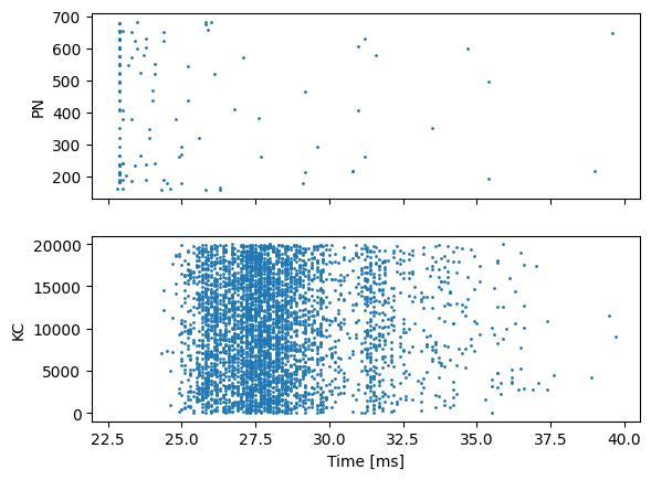
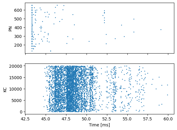
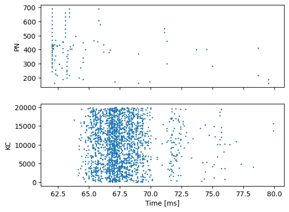
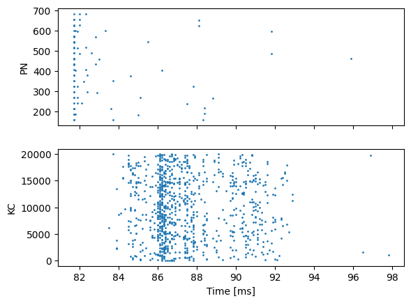
Oh dear! Even with normalised inputs and controlling for the initial state of the model before presenting each stimuli, we get very variable numbers of active Kenyon Cells.