Adding synapses

This tutorial explains how to add synapses to connect the neuron populations we talked about in the previous tutorial into a balanced random network model.

Install PyGeNN wheel from Google Drive

Download wheel file

if "google.colab" in str(get_ipython()):
    #import IPython
    #IPython.core.magics.execution.ExecutionMagics.run.func_defaults[2] = lambda a: a
    #%run "../install_collab.ipynb"
    !pip install gdown --upgrade
    !gdown 1V_GzXUDzcFz9QDIpxAD8QNEglcSipssW
    !pip install pygenn-5.0.0-cp310-cp310-linux_x86_64.whl
    %env CUDA_PATH=/usr/local/cuda

Requirement already satisfied: gdown in /usr/local/lib/python3.10/dist-packages (5.1.0)
Requirement already satisfied: beautifulsoup4 in /usr/local/lib/python3.10/dist-packages (from gdown) (4.12.3)
Requirement already satisfied: filelock in /usr/local/lib/python3.10/dist-packages (from gdown) (3.13.1)
Requirement already satisfied: requests[socks] in /usr/local/lib/python3.10/dist-packages (from gdown) (2.31.0)
Requirement already satisfied: tqdm in /usr/local/lib/python3.10/dist-packages (from gdown) (4.66.2)
Requirement already satisfied: soupsieve>1.2 in /usr/local/lib/python3.10/dist-packages (from beautifulsoup4->gdown) (2.5)
Requirement already satisfied: charset-normalizer<4,>=2 in /usr/local/lib/python3.10/dist-packages (from requests[socks]->gdown) (3.3.2)
Requirement already satisfied: idna<4,>=2.5 in /usr/local/lib/python3.10/dist-packages (from requests[socks]->gdown) (3.6)
Requirement already satisfied: urllib3<3,>=1.21.1 in /usr/local/lib/python3.10/dist-packages (from requests[socks]->gdown) (2.0.7)
Requirement already satisfied: certifi>=2017.4.17 in /usr/local/lib/python3.10/dist-packages (from requests[socks]->gdown) (2024.2.2)
Requirement already satisfied: PySocks!=1.5.7,>=1.5.6 in /usr/local/lib/python3.10/dist-packages (from requests[socks]->gdown) (1.7.1)
Downloading...
From: https://drive.google.com/uc?id=1V_GzXUDzcFz9QDIpxAD8QNEglcSipssW
To: /content/pygenn-5.0.0-cp310-cp310-linux_x86_64.whl
100% 8.29M/8.29M [00:00<00:00, 98.5MB/s]
Processing ./pygenn-5.0.0-cp310-cp310-linux_x86_64.whl
Requirement already satisfied: numpy>=1.17 in /usr/local/lib/python3.10/dist-packages (from pygenn==5.0.0) (1.25.2)
Requirement already satisfied: deprecated in /usr/local/lib/python3.10/dist-packages (from pygenn==5.0.0) (1.2.14)
Requirement already satisfied: psutil in /usr/local/lib/python3.10/dist-packages (from pygenn==5.0.0) (5.9.5)
Requirement already satisfied: wrapt<2,>=1.10 in /usr/local/lib/python3.10/dist-packages (from deprecated->pygenn==5.0.0) (1.14.1)
pygenn is already installed with the same version as the provided wheel. Use --force-reinstall to force an installation of the wheel.
env: CUDA_PATH=/usr/local/cuda

Import numpy, matplotlib and the main GeNNModel class from PyGeNN

import numpy as np
import matplotlib.pyplot as plt

from pygenn import GeNNModel, init_postsynaptic, init_sparse_connectivity, init_var, init_weight_update

Build model

Create a new model called “tutorial2” with floating point precision and set the simulation timestep to 1ms

model = GeNNModel("float", "tutorial2")
model.dt = 1.0

For this tutorial were going to use Leaky-Integrate-and-Fire neurons which have the following dynamics:

:nbsphinx-math:`begin{align}

tau_{text{m}} frac{dV_{i}}{dt} = & (V_{text{rest}} - V_{i}) + R_{text{m}}I_{i}.

end{align}`

We configure these using the parameters from (Vogels & Abbott, 2005 link text). Note that the resting voltage is higher than the reset to provide a constant current input TODO get rid of this

lif_params = {"C": 1.0, "TauM": 20.0, "Vrest": -49.0, "Vreset": -60.0,
              "Vthresh": -50.0, "Ioffset": 0.0, "TauRefrac": 5.0}

So that the network starts in a non-pathological state, we want to randomly initialise the neuron’s membrane potentials so that they are between their threshold and resting potentials. GeNN provides various initialisation “snippets” which can be used to parallelise variable initialisation but, here we are going to use Uniform to sample values from a uniform distribution.

lif_init = {"V": init_var("Uniform", {"min": -60.0, "max": -50.0}),
            "RefracTime": 0.0}

For this tutorial we create an excitary and inhibitory population of these neurons and we enable spike recording for both

exc_pop = model.add_neuron_population("E", 3200, "LIF", lif_params, lif_init)
inh_pop = model.add_neuron_population("I", 800, "LIF", lif_params, lif_init)

exc_pop.spike_recording_enabled = True
inh_pop.spike_recording_enabled = True

So this network sits in a asynchronous irregular state, we initialise the inhibitory weights as follows:

exc_synapse_init = {"g": 0.0008}
inh_synapse_init = {"g": -0.0102}

We are going to use an exponential synapse model where a single time constant \(\tau_{\text{syn}}\) to define it’s dynamics: :nbsphinx-math:`begin{align}

tau_{text{syn}} frac{dI_{text{syn}_{i}}}{dt} = & -I_{text{syn}_{i}} + sum_{j=0}^{n} w_{ij} sum_{t_{j}} delta(t - t_{j}).

end{align}` To approximate biolological AMPA and GABA receptors, we pick different time constants for excitatory and inhibitory synapses.

exc_post_syn_params = {"tau": 5.0}
inh_post_syn_params = {"tau": 10.0}

We want to connect these with a fixed probability of 0.1

fixed_prob = {"prob": 0.1}

Now we have defined the synaptic weights (in GeNN, this is the responsibility of the weight update model), the synapse dynamics (in GeNN this is the responsibility of the postsynaptic model) and the connectivity parameters we can add the synapse populations to the model. Each of these synapse populations all configured with: * SPARSE connectivity meaning that they are connected with a sparse weight matrix. * The built in StaticPulseConstantWeight weight update model which is used for spiking synapses without any sort of learning. This has a single parameter g representing the synaptic weight used for all synapses. * The build in ExpCurr postsynaptic model which implements the exponential synapses described previously * The sparse connectivity is configured using the built in FixedProbability model described previosuly

model.add_synapse_population("EE", "SPARSE",
    exc_pop, exc_pop,
    init_weight_update("StaticPulseConstantWeight", exc_synapse_init),
    init_postsynaptic("ExpCurr", exc_post_syn_params),
    init_sparse_connectivity("FixedProbabilityNoAutapse", fixed_prob))

model.add_synapse_population("EI", "SPARSE",
    exc_pop, inh_pop,
    init_weight_update("StaticPulseConstantWeight", exc_synapse_init),
    init_postsynaptic("ExpCurr", exc_post_syn_params),
    init_sparse_connectivity("FixedProbability", fixed_prob))

model.add_synapse_population("II", "SPARSE",
    inh_pop, inh_pop,
    init_weight_update("StaticPulseConstantWeight", inh_synapse_init),
    init_postsynaptic("ExpCurr", inh_post_syn_params),
    init_sparse_connectivity("FixedProbabilityNoAutapse", fixed_prob))

model.add_synapse_population("IE", "SPARSE",
    inh_pop, exc_pop,
    init_weight_update("StaticPulseConstantWeight", inh_synapse_init),
    init_postsynaptic("ExpCurr", inh_post_syn_params),
    init_sparse_connectivity("FixedProbability", fixed_prob));

Run code generator to generate simulation code for model and load it into PyGeNN. Allocate a spike recording buffer large enough to store the spikes emitted throughout our entire 1 second simulation

model.build()
model.load(num_recording_timesteps=1000)

Simulate model

Simulate the model for 1000 timesteps

while model.timestep < 1000:
    model.step_time()

Copy the recorded spike data back from the GPU and extract the spike times and IDs

model.pull_recording_buffers_from_device()

exc_spike_times, exc_spike_ids = exc_pop.spike_recording_data[0]
inh_spike_times, inh_spike_ids = inh_pop.spike_recording_data[0]

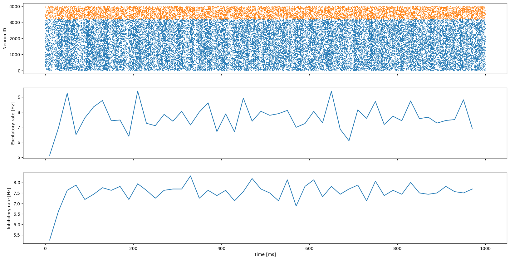
Plot spikes and rates

fig, axes = plt.subplots(3, sharex=True, figsize=(20, 10))

# Define some bins to calculate spike rates
bin_size = 20.0
rate_bins = np.arange(0, 1000.0, bin_size)
rate_bin_centres = rate_bins[:-1] + (bin_size / 2.0)

# Plot excitatory and inhibitory spikes on first axis
axes[0].scatter(exc_spike_times, exc_spike_ids, s=1)
axes[0].scatter(inh_spike_times, inh_spike_ids + 3200, s=1)

# Plot excitatory rates on second axis
exc_rate = np.histogram(exc_spike_times, bins=rate_bins)[0]
axes[1].plot(rate_bin_centres, exc_rate * (1000.0 / bin_size) * (1.0 / 3200.0))

# Plot inhibitory rates on third axis
inh_rate = np.histogram(inh_spike_times, bins=rate_bins)[0]
axes[2].plot(rate_bin_centres, inh_rate * (1000.0 / bin_size) * (1.0 / 800.0))

# Label axes
axes[0].set_ylabel("Neuron ID")
axes[1].set_ylabel("Excitatory rate [Hz]")
axes[2].set_ylabel("Inhibitory rate [Hz]")
axes[2].set_xlabel("Time [ms]");